


Will Degrees Magnetic be eliminated eventually?

Join Date: Apr 2006
Location: Vietnam
Posts: 29
Likes: 0
Received 0 Likes
on
0 Posts
The obvious place to start is with the fundamental assertion of the book Origin and Destiny of the Earth's Magnetic Field by Thomas G. Barnes, I.C.R. Technical Monograph No. 4, copyright July, 1973, by the Institute for Creation Research. Barnes earned an A.B. degree in physics from Hardin-Simmons College, that the Earth's magnetic field is exponentially decaying. If this turns out to be untrue, or unsupportable, then Barnes' entire thesis is immediately nullified. So the next most obvious thing to do at this point is to present the reader with the data. These data, which follow in my table 2, are taken from Barnes (pages 33 & 61). Barnes in turn credits the ESSA report of McDonald & Gunst [5] as his source. I once saw a copy of that report, but am not able to find it now. I presume that Barnes can copy, and that the data are as given in [5]. In any case, these are the data that Barnes presents in defence of his own thesis, so the enterprising reader can examine the data as they see fit, in order to gauge compliance with the exponential decay hypothesis. Multiple values for one year indicate separate determinations, reported in separate original references. Those references are given by Barnes, but I have omitted them here.
Table 2
Dipole Magnetic Moment Data
From Barnes Pages 33 & 61 Year Dipole Moment
(� 1022 amp-meter2)1835 8.5581845 8.4881880 8.3631880 8.3361885 8.3471885 8.3751905 8.2911915 8.2251922 8.1651925 8.1491935 8.0881942.58.0091945 8.0651945 8.0101945 8.0661945 8.0901955 8.0351955 8.0671958.58.0381959 8.0861960 8.0531960 8.0371960 8.0251965 8.0131965 8.017Before we go any farther, the attentive reader should have already spotted at least one problem. This table does not show any experimental uncertainties associated with any of the data points. This is the manner in which Barnes presents the data, and nowhere in his book is the subject of experimental uncertainty mentioned at all. I have not seen the McDonald & Gunst paper in preparing this article, so I cannot say whether or not they presented the data without uncertainties as well, but if they did, then their own argument suffers from the omission just as Barnes' argument does here.
From these data Barnes has determined that the Earth's magnetic field is decaying exponentially. Throughout his book, whenever he mentions this exponential decay, he points the reader to section II-D, page 36 to view the justification. On that page of his book, he justifies the exponential decay conclusion as follows, the emphasis is mine. B0, as referred to by Barnes, is the equatorial magnetic field strength, which is included in his tables, but omitted from mine.
Even without a plot, just by looking at the data tabulated above, the reader should be able to see that the moment values since 1935 appear essentially flat around a value of about 8.047 +/- 0.029, while the data prior to 1935 show a clear downward trend. One could easily argue that two straight lines fit the data better than one, and even better than one exponential (this is an exercise that I have not undertaken, but the motivated reader is welcome to see if my intuition is trustworthy). That fact alone will easily explain why a single exponential will fit the data better than a single straight line, as the slight curve of the exponential can better approximate the kink in the data. These considerations make it extremely difficult to use the data alone as an a-priori justification for any particular curve fit over another. In fact, one could over interpret the data even to the extent of claiming that the field was in decay until about 1935, when it then stopped decaying.
Table 2
Dipole Magnetic Moment Data
From Barnes Pages 33 & 61 Year Dipole Moment
(� 1022 amp-meter2)1835 8.5581845 8.4881880 8.3631880 8.3361885 8.3471885 8.3751905 8.2911915 8.2251922 8.1651925 8.1491935 8.0881942.58.0091945 8.0651945 8.0101945 8.0661945 8.0901955 8.0351955 8.0671958.58.0381959 8.0861960 8.0531960 8.0371960 8.0251965 8.0131965 8.017Before we go any farther, the attentive reader should have already spotted at least one problem. This table does not show any experimental uncertainties associated with any of the data points. This is the manner in which Barnes presents the data, and nowhere in his book is the subject of experimental uncertainty mentioned at all. I have not seen the McDonald & Gunst paper in preparing this article, so I cannot say whether or not they presented the data without uncertainties as well, but if they did, then their own argument suffers from the omission just as Barnes' argument does here.
From these data Barnes has determined that the Earth's magnetic field is decaying exponentially. Throughout his book, whenever he mentions this exponential decay, he points the reader to section II-D, page 36 to view the justification. On that page of his book, he justifies the exponential decay conclusion as follows, the emphasis is mine. B0, as referred to by Barnes, is the equatorial magnetic field strength, which is included in his tables, but omitted from mine.
"When values of the magnetic moment, M, in table 1 are plotted against time, t, on semi-log coordinate paper, the points lie approximately on a straight line, as one would expect for an exponential decay of the Earth's magnetic moment. This is also true, of course, for a plot of B0 against t. We therefore assume that the decay is exponential and write ... "
This, of course, is no justification at all. Barnes simply assumed that the decay was exponential. However, later in the book, at the beginning of section IV, page 52, Barnes makes a slightly more heroic attempt to justify the exponential decay theory as follows:"All data were processed on a CDC3100 electronic computer. A least square exponential fit was employed to evaluate the time constant. As a separate check it was noted that the variability was smaller for this exponential fit than for a straight line fit, as one would expect from the exponential solutions obtained from Maxwell's equations."
In these two passages we see the full and entire text of the justification for deriving an exponential decay from the tabulated data. Anyone reading this who has had experience with numerical approximations, data curve fitting, and etc. should be able to recognize at once that the argument is very poor. First, it should be obvious that one cannot perform an unweighted fit, completely ignoring any experimental uncertainties. The early data from the mid 1800's, which are derived from experimental methods that are far less accurate and precise than modern methods, necessarily have much larger uncertainties associated with them, and should be weighted accordingly in any attempt to fit the data to a curve. Second, Barnes' reference to the "variability" of the exponential versus straight line fit is highly ambiguous. Is "variability" supposed to mean "variance"? If the variance of the fit is greater than the experimental uncertainties, then the line and exponential cannot be distinguished, in fact, one from the other. And what does "smaller" mean? Was the difference in variance between the two fits (if that is what "variability" means) significant or not? These kinds of curve fitting exercises are fraught with peril, and relying on the difference in variance between fits, where it is obvious that in fact either an exponential or a straight line will produce a "good" fit, is an exceptionally unreliable procedure.Even without a plot, just by looking at the data tabulated above, the reader should be able to see that the moment values since 1935 appear essentially flat around a value of about 8.047 +/- 0.029, while the data prior to 1935 show a clear downward trend. One could easily argue that two straight lines fit the data better than one, and even better than one exponential (this is an exercise that I have not undertaken, but the motivated reader is welcome to see if my intuition is trustworthy). That fact alone will easily explain why a single exponential will fit the data better than a single straight line, as the slight curve of the exponential can better approximate the kink in the data. These considerations make it extremely difficult to use the data alone as an a-priori justification for any particular curve fit over another. In fact, one could over interpret the data even to the extent of claiming that the field was in decay until about 1935, when it then stopped decaying.


Join Date: Dec 2005
Location: UK
Posts: 644
Likes: 0
Received 0 Likes
on
0 Posts
Arismount,
I hear you dude and yes the point is taken. But this kind of comedy happens from time. Nevertheless the magnetic pole debate is quite interesting let's get back to that seeing as we're all happy buddies again
I hear you dude and yes the point is taken. But this kind of comedy happens from time. Nevertheless the magnetic pole debate is quite interesting let's get back to that seeing as we're all happy buddies again
Thread Starter
Join Date: Jul 2005
Location: Canada
Posts: 30
Likes: 0
Received 0 Likes
on
0 Posts
Originally Posted by bookworm
I think you (or possibly the textbook's authors) are missing the point. In the sat-nav future, once you have a system that tells you where you are and knows where you need to be, the arbitrary zero reference of your direction measure is irrelevant. An autopilot will fly from A to B just as well on magnetic or true, measured in degrees, grades or radians. The concept of flying a particular published track or heading loses its relevance, because you're always flying to an endpoint, regardless of the direction that happens to be.
In the mean time, we might as well pick the easiest/cheapest possibility as the zero reference for purposes like ATC telling you which direction to point your aircraft. That easiest/cheapest possibility probably remains magnetic north.
In the mean time, we might as well pick the easiest/cheapest possibility as the zero reference for purposes like ATC telling you which direction to point your aircraft. That easiest/cheapest possibility probably remains magnetic north.
It would seem to me radio-nav won't have much use left either.
Join Date: Apr 2006
Location: Vietnam
Posts: 29
Likes: 0
Received 0 Likes
on
0 Posts
Calculation of new positional information, which is based on both GPS and dead reckoning data, then takes place in a so-called "Kalman filter." At this location, the evaluation and combination of these data occur, including the previous history. Because processed GPS data enter the Kalman filter, i.e. values calculated for longitude, latitude and direction, one speaks of a loosely controlled system. The calculation of GPS data also already occurred via a Kalman filter.
Besides this implementation of a loose system with feedback, other loose systems exist without feedback (the dead-reckoning signals are not calibrated), as well as tightly controlled systems with or without feedback. In tightly controlled systems, raw GPS data, i.e. pseudo-ranges and delta ranges, are processed into a single Kalman filter, instead of the GPS data being processed first by their own Kalman filter. Because the Kalman filter makes up the heart of the calculations, we should briefly explain the principles behind it......
A Linear Dynamical System is a partially observed stochastic process with linear dynamics and linear observations, both subject to Gaussian noise. It can be defined as follows, where X(t) is the hidden state at time t, and Y(t) is the observation. x(t+1) = F*x(t) + w(t), w ~ N(0, Q), x(0) ~ N(X(0), V(0)) y(t) = H*x(t) + v(t), v ~ N(0, R)The Kalman filter is an algorithm for performing filtering on this model, i.e., computing P(X(t) | Y(1), ..., Y(t)).
The Rauch-Tung-Striebel (RTS) algorithm performs fixed-interval offline smoothing, i.e., computing P(X(t) | Y(1), ..., Y(T)), for t <= T.
Here is a simple example. Consider a particle moving in the plane at constant velocity subject to random perturbations in its trajectory. The new position (x1, x2) is the old position plus the velocity (dx1, dx2) plus noise w.
[ x1(t) ] = [1 0 1 0] [ x1(t-1) ] + [ wx1 ][ x2(t) ] [0 1 0 1] [ x2(t-1) ] [ wx2 ][ dx1(t) ] [0 0 1 0] [ dx1(t-1) ] [ wdx1 ][ dx2(t) ] [0 0 0 1] [ dx2(t-1) ] [ wdx2 ]We assume we only observe the position of the particle.
[ y1(t) ] = [1 0 0 0] [ x1(t) ] + [ vx1 ][ y2(t) ] [0 1 0 0] [ x2(t) ] [ vx2 ] [ dx1(t) ] [ dx2(t) ]Suppose we start out at position (10,10) moving to the right with velocity (1,0). We sampled a random trajectory of length 15.
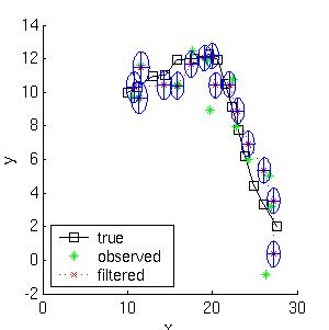
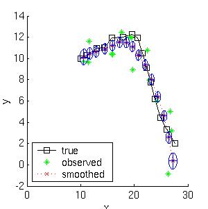 The mean squared error of the filtered estimate is 4.9; for the smoothed estimate it is 3.2. Not only is the smoothed estimate better, but we know that it is better, as illustrated by the smaller uncertainty ellipses; this can help in e.g., data association problems. Note how the smoothed ellipses are larger at the ends, because these points have seen less data. Also, note how rapidly the filtered ellipses reach their steady-state (Ricatti) values.
Directional input from GPS become inaccurate at low speeds until it loses all meaning at a standstill. This is a fact that one must consider. Therefore below a certain speed, the directional information from the gyro should be taken more strongly into consideration; at standstill the directional information should not be recalculated. At the same time, the standstill state should be utilized to reset the gyro's open-circuit voltage. Especially in cities, where dead reckoning is deployed more often than in open space due to gaps between buildings or tunnels, stops at traffic signals can be used for this purpose. Deviations are thereby reduced.
Besides this implementation of a loose system with feedback, other loose systems exist without feedback (the dead-reckoning signals are not calibrated), as well as tightly controlled systems with or without feedback. In tightly controlled systems, raw GPS data, i.e. pseudo-ranges and delta ranges, are processed into a single Kalman filter, instead of the GPS data being processed first by their own Kalman filter. Because the Kalman filter makes up the heart of the calculations, we should briefly explain the principles behind it......
A Linear Dynamical System is a partially observed stochastic process with linear dynamics and linear observations, both subject to Gaussian noise. It can be defined as follows, where X(t) is the hidden state at time t, and Y(t) is the observation. x(t+1) = F*x(t) + w(t), w ~ N(0, Q), x(0) ~ N(X(0), V(0)) y(t) = H*x(t) + v(t), v ~ N(0, R)The Kalman filter is an algorithm for performing filtering on this model, i.e., computing P(X(t) | Y(1), ..., Y(t)).
The Rauch-Tung-Striebel (RTS) algorithm performs fixed-interval offline smoothing, i.e., computing P(X(t) | Y(1), ..., Y(T)), for t <= T.
Here is a simple example. Consider a particle moving in the plane at constant velocity subject to random perturbations in its trajectory. The new position (x1, x2) is the old position plus the velocity (dx1, dx2) plus noise w.
[ x1(t) ] = [1 0 1 0] [ x1(t-1) ] + [ wx1 ][ x2(t) ] [0 1 0 1] [ x2(t-1) ] [ wx2 ][ dx1(t) ] [0 0 1 0] [ dx1(t-1) ] [ wdx1 ][ dx2(t) ] [0 0 0 1] [ dx2(t-1) ] [ wdx2 ]We assume we only observe the position of the particle.
[ y1(t) ] = [1 0 0 0] [ x1(t) ] + [ vx1 ][ y2(t) ] [0 1 0 0] [ x2(t) ] [ vx2 ] [ dx1(t) ] [ dx2(t) ]Suppose we start out at position (10,10) moving to the right with velocity (1,0). We sampled a random trajectory of length 15.
The mean squared error of the filtered estimate is 4.9; for the smoothed estimate it is 3.2. Not only is the smoothed estimate better, but we know that it is better, as illustrated by the smaller uncertainty ellipses; this can help in e.g., data association problems. Note how the smoothed ellipses are larger at the ends, because these points have seen less data. Also, note how rapidly the filtered ellipses reach their steady-state (Ricatti) values.Directional input from GPS become inaccurate at low speeds until it loses all meaning at a standstill. This is a fact that one must consider. Therefore below a certain speed, the directional information from the gyro should be taken more strongly into consideration; at standstill the directional information should not be recalculated. At the same time, the standstill state should be utilized to reset the gyro's open-circuit voltage. Especially in cities, where dead reckoning is deployed more often than in open space due to gaps between buildings or tunnels, stops at traffic signals can be used for this purpose. Deviations are thereby reduced.
Join Date: Aug 2005
Location: Charlotte and NYC
Age: 45
Posts: 53
Likes: 0
Received 0 Likes
on
0 Posts

Do the JAA know about this????
Seriously though, its actually inspiring to see things discussed in depth. Can anyone recommend a good (in depth) text on GPS? Using it is one thing, but it is nice to know whats actually going on in the equipment.
Join Date: Mar 2006
Location: Finland - East of Sweden
Posts: 113
Likes: 0
Received 0 Likes
on
0 Posts
How do people feel about the EU's Galileo GPS program? It's being sold as a significant improvement, offering an unforeseen redundancy to the use of public satellite positioning systems, including aviation uses. A me-too or what?
Join Date: Jun 2004
Location: UK
Posts: 172
Likes: 0
Received 0 Likes
on
0 Posts
Originally Posted by CashKing
Especially in cities, where dead reckoning is deployed more often than in open space due to gaps between buildings or tunnels, stops at traffic signals can be used for this purpose. Deviations are thereby reduced.
Pasted text from a web site about car navigation systems notwithstanding, I expect that Kalman filter algorithms are used in FMCs when combining data from multiple sensors (gps, dme, irs etc.) to generate a composite FMC position. Not sure about the relevance to GPS per se?
As to the original question, GPS cannot provide heading. It can only provide track and then only when moving. An AHRS can provide true heading, so you really need combined GPS / AHRS to be independant of the earth's magnetism. When all aircraft can have a combined GPS / AHRS costing less than current instruments we may see a switch to true navigation.
Last edited by Rivet gun; 22nd Apr 2006 at 19:37.
Join Date: Apr 2006
Location: Vietnam
Posts: 29
Likes: 0
Received 0 Likes
on
0 Posts
The applications are endless. Kalman filtering has proved useful in navigational and guidance systems, radar tracking, sonar ranging, and satellite orbit determination, to name just a few areas. Anything that moves, if it's automated, is a candidate for a Kalman filter.
